New research on social media during the 2020 election, and my predictions
This is crossposted from Statistical Modeling, Causal Inference, and Social Science.
Back in 2020, leading academics and researchers at the company now known as Meta put together a large project to study social media and the 2020 US elections — particularly the roles of Instagram and Facebook. As Sinan Aral and I had written about how many paths for understanding effects of social media in elections could require new interventions and/or platform cooperation, this seemed like an important development. Originally the idea was for this work to be published in 2021, but there have been some delays, including simply because some of the data collection was extended as what one might call “election-related events” continued beyond November and into 2021. As of 2pm Eastern today, the news embargo for this work has been lifted on the first group of research papers.
I had heard about this project back a long time ago and, frankly, had largely forgotten about it. But this past Saturday, I was participating in the SSRC Workshop on the Economics of Social Media and one session was dedicated to results-free presentations about this project, including the setup of the institutions involved and the design of the research. The organizers informally polled us with qualitative questions about some of the results. This intrigued me. I had recently reviewed an unrelated paper that included survey data from experts and laypeople about their expectations about the effects estimated in a field experiment, and I thought this data was helpful for contextualizing what “we” learned from that study.
So I thought it might be useful, at least for myself, to spend some time eliciting my own expectations about the quantities I understood would be reported in these papers. I’ve mainly kept up with the academic and grey literature, I’d previously worked in the industry, and I’d reviewed some of this for my Senate testimony back in 2021. Along the way, I tried to articulate where my expectations and remaining uncertainty were coming from. I composed many of my thoughts on my phone Monday while taking the subway to and from the storage unit I was revisiting and then emptying in Brooklyn. I got a few comments from Solomon Messing and Tom Cunningham, and then uploaded my notes to OSF and posted a cheeky tweet.
Since then, starting yesterday, I’ve spoken with journalists and gotten to view the main text of papers for two of the randomized interventions for which I made predictions. These evaluated effects of (a) switching Facebook and Instagram users to a (reverse) chronological feed, (b) removing “reshares” from Facebook users’ feeds, and (c) downranking content by “like-minded” users, Pages, and Groups.
My guesses
My main expectations for those three interventions could be summed up as follows. These interventions, especially chronological ranking, would each reduce engagement with Facebook or Instagram. This makes sense if you think the status quo is somewhat-well optimized for showing engaging and relevant content. So some of the rest of the effects — on, e.g., polarization, news knowledge, and voter turnout — could be partially inferred from that decrease in use. This would point to reductions in news knowledge, issue polarization (or coherence/consistency), and small decreases in turnout, especially for chronological ranking. This is because people get some hard news and political commentary they wouldn’t have otherwise from social media. These reduced-engagement-driven effects should be weakest for the “soft” intervention of downranking some sources, since content predicted to be particularly relevant will still make it into users’ feeds.
Besides just reducing Facebook use (and everything that goes with that), I also expected swapping out feed ranking for reverse chron would expose users to more content from non-friends via, e.g., Groups, including large increases in untrustworthy content that would normally rank poorly. I expected some of the same would happen from removing reshares, which I expected would make up over 20% of views under the status quo, and so would be filled in by more Groups content. For downranking sources with the same estimated ideology, I expected this would reduce exposure to political content, as much of the non-same-ideology posts will be by sources with estimated ideology in the middle of the range, i.e. [0.4, 0.6], which are less likely to be posting politics and hard news. I’ll also note that much of my uncertainty about how chronological ranking would perform was because there were a lot of unknown but important “details” about implementation, such as exactly how much of the ranking system really gets turned off (e.g., how much likely spam/scam content still gets filtered out in an early stage?).
How’d I do?
Here’s a quick summary of my guesses and the results in these three papers:
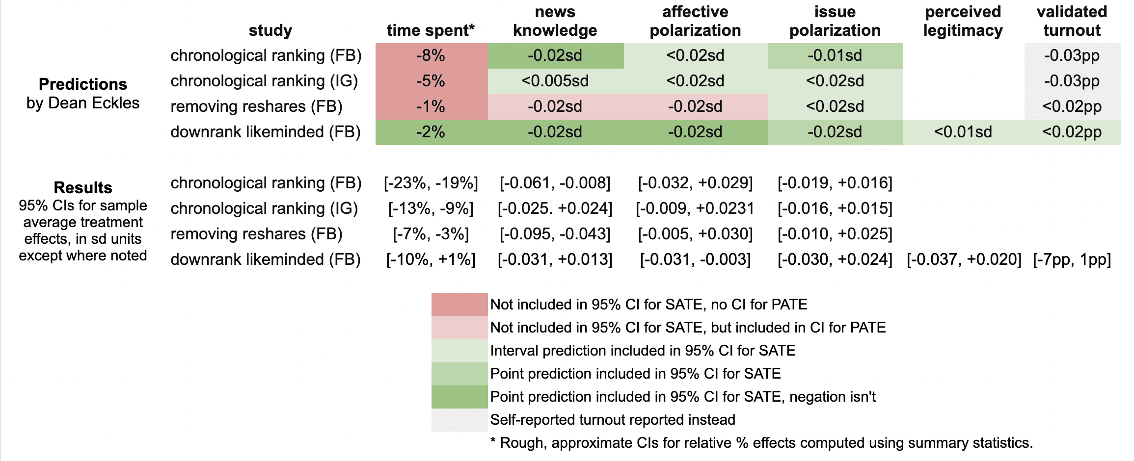
It looks like I was wrong in that the reductions in engagement were larger than I predicted: e.g., chronological ranking reduced time spent on Facebook by 21%, rather than the 8% I guessed, which was based on my background knowledge, a leaked report on a Facebook experiment, and this published experiment from Twitter.
Ex post I hypothesize that this is because of the duration of these experiments allowed for continual declines in use over months, with various feedback loops (e.g., users with chronological feed log in less, so they post less, so they get fewer likes and comments, so they log in even less and post even less). As I dig into the 100s of pages of supplementary materials, I’ll be looking to understand what these declines looked like at earlier points in the experiment, such as by election day.
My estimates for the survey-based outcomes of primary interest, such as polarization, were mainly covered by the 95% confidence intervals, with the exception of two outcomes from the “no reshares” intervention.
One thing is that all these papers report weighted estimates for a broader population of US users (population average treatment effects, PATEs), which are less precise than the unweighted (sample average treatment effect, SATE) results. Here I focus mainly on the unweighted results, as I did not know there was going to be any weighting and these are also the more narrow, and thus riskier, CIs for me. (There seems to have been some mismatch between the outcomes listed in the talk I saw and what’s in the papers, so I didn’t make predictions for some reported primary outcomes and some outcomes I made predictions for don’t seem to be reported, or I haven’t found them in the supplements yet.)
Now is a good time to note that I basically predicted what psychologists armed with Jacob Cohen’s rules of thumb might call extrapolate to “minuscule” effect sizes. All my predictions for survey-based outcomes were 0.02 standard deviations or smaller. (Recall Cohen’s rules of thumb say 0.1 is small, 0.5 medium, and 0.8 large.)
Nearly all the results for these outcomes in these two papers were indistinguishable from the null (p > 0.05), with standard errors for survey outcomes at 0.01 SDs or more. This is consistent with my ex ante expectations that the experiments would face severe power problems, at least for the kind of effects I would expect. Perhaps by revealed preference, a number of other experts had different priors.
A rare p < 0.05 result is that that chronological ranking reduced news knowledge by 0.035 SDs with 95% CI [-0.061, -0.008], which includes my guess of -0.02 SDs. Removing reshares may have reduced news knowledge even more than chronological ranking — and by more than I guessed.
Even with so many null results I was still sticking my neck out a bit compared with just guessing zero everywhere, since in some cases if I had put the opposite sign my estimate wouldn’t have been in the 95% CI. For example, downranking “like-minded” sources produced a CI of [-0.031, 0.013] SDs, which includes my guess of -0.02, but not its negation. On the other hand, I got some of these wrong, where I guessed removing reshares would reduce affective polarization, but a 0.02 SD effect is outside the resulting [-0.005, +0.030] interval.
It was actually quite a bit of work to compare my predictions to the results because I didn’t really know a lot of key details about exact analyses and reporting choices, which strikingly even differ a bit across these three papers. So I might yet find more places where I can, with a lot of reading and a bit of arithmetic, figure out where else I may have been wrong. (Feel free to point these out.)
Further reflections
I hope that this helps to contextualize the present results with expert consensus — or at least my idiosyncratic expectations. I’ll likely write a bit more about these new papers and further work released as part of this project.
It was probably an oversight for me not to make any predictions about the observational paper looking at polarization in exposure and consumption of news media. I felt like I had a better handle on thinking about simple treatment effects than these measures, but perhaps that was all the more reason to make predictions. Furthermore, given the limited precision of the experiments’ estimates, perhaps it would have been more informative (and riskier) to make point predictions about these precisely estimated observational quantities.
[I want to note that I was an employee or contractor of Facebook (now Meta) from 2010 through 2017. I have received funding for other research from Meta, Meta has sponsored a conference I organize, and I have coauthored with Meta employees as recently as earlier this month. I was also recently a consultant to Twitter, ending shortly after the Musk acquisition. You can find all my disclosures here.]
Against between-subjects experiments
A less widely known reason for using within-subjects experimental designs in psychological science. In a within-subjects experiment, each participant experiences multiple conditions (say, multiple persuasive messages), while in a between-subjects experiment, each participant experiences only one condition.
If you ask a random social psychologist, “Why would you run a within-subjects experiment instead of a between-subjects experiments?”, the most likely answer is “power” — within-subjects experiments provide more power. That is, with the same number of participants, within-subjects experiments allow investigators to more easily tell that observed differences between conditions are not due to chance. ((And to more precisely estimate these differences. Though social psychologist often don’t care about estimation, since many social psychological theories are only directional.))
Why do within-subjects experiments increase power? Because responses by the same individual are generally dependent; more specifically, they are often positively correlated. Say an experiment involves evaluating products, people, or policy proposals under different conditions, such as the presence of different persuasive cues or following different primes. It is often the case that participants who rate an item high on a scale under one condition will rate other items high on that scale under other condition. Or participants with short response times for one task will have relatively short response times for another task. Et cetera. This positive association might be due to stable characteristics of people or transient differences such as mood. Thus, the increase in power is due to heterogeneity in how individuals respond to the stimuli.
However, this advantage of within-subjects designs is frequently overridden in social psychology by the appeal of between-subjects designs. The latter are widely regarded as “cleaner” as they avoid carryover effects — in which one condition may effect responses to subsequent conditions experienced by the same participant. They can also be difficult to design when studies involve deception — even just deception about the purpose of the study — and one-shot encounters. Because of this, between-subjects designs are much more common in social psychology than within-subjects designs: investigators don’t regard the complexity of conducting within-subjects designs as worth it for the gain in power, which they regard as the primary advantage of within-subjects designs.
I want to point out another — but related — reason for using within-subjects designs: between-subjects experiments often do not allow consistent estimation of the parameters of interest. Now, between-subjects designs are great for estimating average treatment effects (ATEs), and ATEs can certainly be of great interest. For example, if one is interested how a design change to a web site will effect sales, an ATE estimated from an A-B test with the very same population will be useful. But this isn’t enough for psychological science for two reasons. First, social psychology experiments are usually very different from the circumstances of potential application: the participants are undergraduate students in psychology and the manipulations and situations are not realistic. So the ATE from a psychology experiment might not say much about the ATE for a real intervention. Second, social psychologists regard themselves as building and testing theories about psychological processes. By their nature, psychological processes occur within individuals. So an ATE won’t do — in fact, it can be a substantially biased estimate of the psychological parameter of interest.
To illustrate this problem, consider an example where the outcome of an experiment is whether the participant says that a job candidate should be hired. For simplicity, let’s say this is a binary outcome: either they say to hire them or not. Their judgements might depend on some discrete scalar X. Different participants may have different thresholds for hiring the applicant, but otherwise be effected by X in the same way. In a logistic model, that is, each participant has their own intercept but all the slopes are the same. This is depicted with the grey curves below. ((This example is very directly inspired by Alan Agresti’s Categorical Data Analysis, p. 500.))

These grey curves can be estimated if one has multiple observations per participant at different values of X. However, in a between-subjects experiment, this is not the case. As an estimate of a parameter of the psychological process common to all the participants, the estimated slope from a between-subjects experiment will be biased. This is clear in the figure above: the blue curve (the marginal expectation function) is shallower than any of the individual curves.
More generally, between-subjects experiments are good for estimating ATEs and making striking demonstrations. But they are often insufficient for investigating psychological processes since any heterogeneity — even only in intercepts — produces biased estimates of the parameters of psychological processes, including parameters that are universal in the population.
I see this as a strong motivation for doing more within-subjects experiments in social psychology. Unlike the power motivation for within-subjects designs, this isn’t solved by getting a larger sample of individuals. Instead, investigators need to think carefully about whether their experiments estimate any quantity of interest when there is substantial heterogeneity — as there generally is. ((The situation is made a bit “better” by the fact that social psychologists are often only concerned with determining the direction of effects, so maybe aren’t worried that their estimates of parameters are biased. Of course, this is a problem in itself if the direction of the effect varies by individual. Here I have only treated the simpler case of universal function subject to a random shift.))