New research on social media during the 2020 election, and my predictions
This is crossposted from Statistical Modeling, Causal Inference, and Social Science.
Back in 2020, leading academics and researchers at the company now known as Meta put together a large project to study social media and the 2020 US elections — particularly the roles of Instagram and Facebook. As Sinan Aral and I had written about how many paths for understanding effects of social media in elections could require new interventions and/or platform cooperation, this seemed like an important development. Originally the idea was for this work to be published in 2021, but there have been some delays, including simply because some of the data collection was extended as what one might call “election-related events” continued beyond November and into 2021. As of 2pm Eastern today, the news embargo for this work has been lifted on the first group of research papers.
I had heard about this project back a long time ago and, frankly, had largely forgotten about it. But this past Saturday, I was participating in the SSRC Workshop on the Economics of Social Media and one session was dedicated to results-free presentations about this project, including the setup of the institutions involved and the design of the research. The organizers informally polled us with qualitative questions about some of the results. This intrigued me. I had recently reviewed an unrelated paper that included survey data from experts and laypeople about their expectations about the effects estimated in a field experiment, and I thought this data was helpful for contextualizing what “we” learned from that study.
So I thought it might be useful, at least for myself, to spend some time eliciting my own expectations about the quantities I understood would be reported in these papers. I’ve mainly kept up with the academic and grey literature, I’d previously worked in the industry, and I’d reviewed some of this for my Senate testimony back in 2021. Along the way, I tried to articulate where my expectations and remaining uncertainty were coming from. I composed many of my thoughts on my phone Monday while taking the subway to and from the storage unit I was revisiting and then emptying in Brooklyn. I got a few comments from Solomon Messing and Tom Cunningham, and then uploaded my notes to OSF and posted a cheeky tweet.
Since then, starting yesterday, I’ve spoken with journalists and gotten to view the main text of papers for two of the randomized interventions for which I made predictions. These evaluated effects of (a) switching Facebook and Instagram users to a (reverse) chronological feed, (b) removing “reshares” from Facebook users’ feeds, and (c) downranking content by “like-minded” users, Pages, and Groups.
My guesses
My main expectations for those three interventions could be summed up as follows. These interventions, especially chronological ranking, would each reduce engagement with Facebook or Instagram. This makes sense if you think the status quo is somewhat-well optimized for showing engaging and relevant content. So some of the rest of the effects — on, e.g., polarization, news knowledge, and voter turnout — could be partially inferred from that decrease in use. This would point to reductions in news knowledge, issue polarization (or coherence/consistency), and small decreases in turnout, especially for chronological ranking. This is because people get some hard news and political commentary they wouldn’t have otherwise from social media. These reduced-engagement-driven effects should be weakest for the “soft” intervention of downranking some sources, since content predicted to be particularly relevant will still make it into users’ feeds.
Besides just reducing Facebook use (and everything that goes with that), I also expected swapping out feed ranking for reverse chron would expose users to more content from non-friends via, e.g., Groups, including large increases in untrustworthy content that would normally rank poorly. I expected some of the same would happen from removing reshares, which I expected would make up over 20% of views under the status quo, and so would be filled in by more Groups content. For downranking sources with the same estimated ideology, I expected this would reduce exposure to political content, as much of the non-same-ideology posts will be by sources with estimated ideology in the middle of the range, i.e. [0.4, 0.6], which are less likely to be posting politics and hard news. I’ll also note that much of my uncertainty about how chronological ranking would perform was because there were a lot of unknown but important “details” about implementation, such as exactly how much of the ranking system really gets turned off (e.g., how much likely spam/scam content still gets filtered out in an early stage?).
How’d I do?
Here’s a quick summary of my guesses and the results in these three papers:
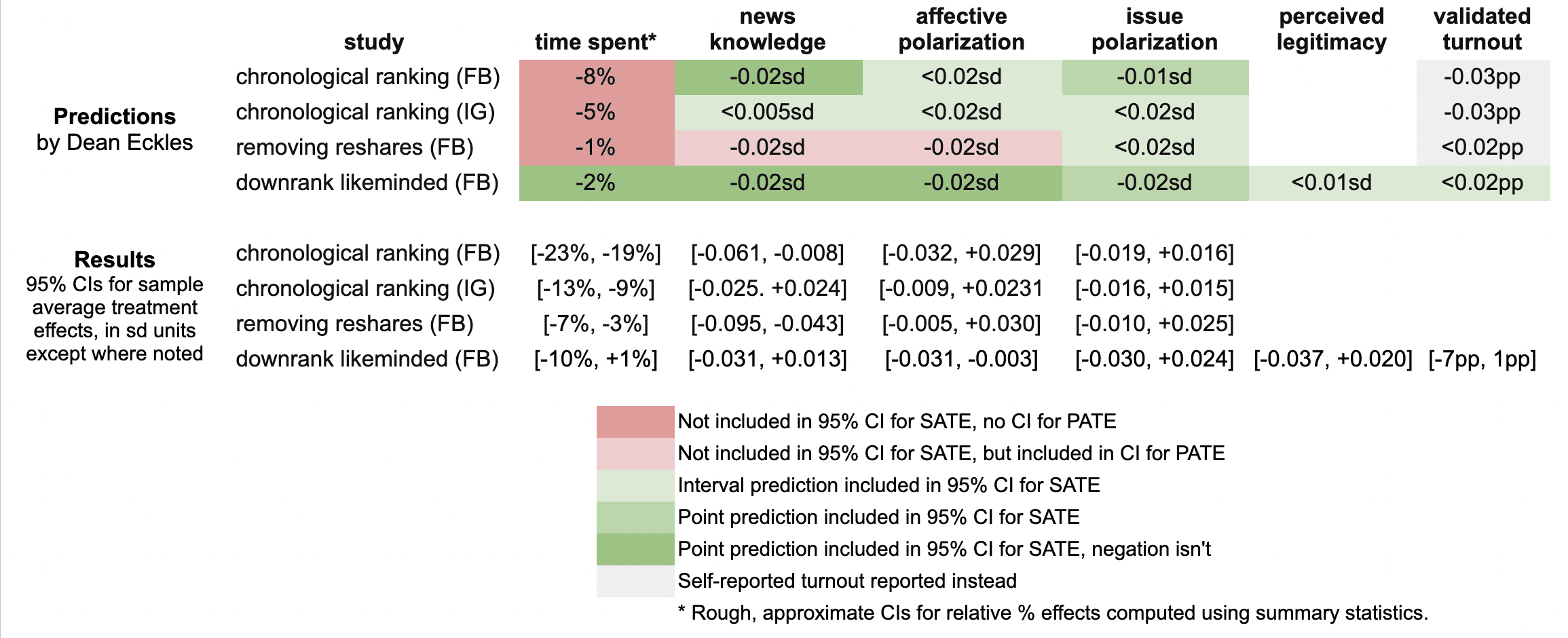
It looks like I was wrong in that the reductions in engagement were larger than I predicted: e.g., chronological ranking reduced time spent on Facebook by 21%, rather than the 8% I guessed, which was based on my background knowledge, a leaked report on a Facebook experiment, and this published experiment from Twitter.
Ex post I hypothesize that this is because of the duration of these experiments allowed for continual declines in use over months, with various feedback loops (e.g., users with chronological feed log in less, so they post less, so they get fewer likes and comments, so they log in even less and post even less). As I dig into the 100s of pages of supplementary materials, I’ll be looking to understand what these declines looked like at earlier points in the experiment, such as by election day.
My estimates for the survey-based outcomes of primary interest, such as polarization, were mainly covered by the 95% confidence intervals, with the exception of two outcomes from the “no reshares” intervention.
One thing is that all these papers report weighted estimates for a broader population of US users (population average treatment effects, PATEs), which are less precise than the unweighted (sample average treatment effect, SATE) results. Here I focus mainly on the unweighted results, as I did not know there was going to be any weighting and these are also the more narrow, and thus riskier, CIs for me. (There seems to have been some mismatch between the outcomes listed in the talk I saw and what’s in the papers, so I didn’t make predictions for some reported primary outcomes and some outcomes I made predictions for don’t seem to be reported, or I haven’t found them in the supplements yet.)
Now is a good time to note that I basically predicted what psychologists armed with Jacob Cohen’s rules of thumb might call extrapolate to “minuscule” effect sizes. All my predictions for survey-based outcomes were 0.02 standard deviations or smaller. (Recall Cohen’s rules of thumb say 0.1 is small, 0.5 medium, and 0.8 large.)
Nearly all the results for these outcomes in these two papers were indistinguishable from the null (p > 0.05), with standard errors for survey outcomes at 0.01 SDs or more. This is consistent with my ex ante expectations that the experiments would face severe power problems, at least for the kind of effects I would expect. Perhaps by revealed preference, a number of other experts had different priors.
A rare p < 0.05 result is that that chronological ranking reduced news knowledge by 0.035 SDs with 95% CI [-0.061, -0.008], which includes my guess of -0.02 SDs. Removing reshares may have reduced news knowledge even more than chronological ranking — and by more than I guessed.
Even with so many null results I was still sticking my neck out a bit compared with just guessing zero everywhere, since in some cases if I had put the opposite sign my estimate wouldn’t have been in the 95% CI. For example, downranking “like-minded” sources produced a CI of [-0.031, 0.013] SDs, which includes my guess of -0.02, but not its negation. On the other hand, I got some of these wrong, where I guessed removing reshares would reduce affective polarization, but a 0.02 SD effect is outside the resulting [-0.005, +0.030] interval.
It was actually quite a bit of work to compare my predictions to the results because I didn’t really know a lot of key details about exact analyses and reporting choices, which strikingly even differ a bit across these three papers. So I might yet find more places where I can, with a lot of reading and a bit of arithmetic, figure out where else I may have been wrong. (Feel free to point these out.)
Further reflections
I hope that this helps to contextualize the present results with expert consensus — or at least my idiosyncratic expectations. I’ll likely write a bit more about these new papers and further work released as part of this project.
It was probably an oversight for me not to make any predictions about the observational paper looking at polarization in exposure and consumption of news media. I felt like I had a better handle on thinking about simple treatment effects than these measures, but perhaps that was all the more reason to make predictions. Furthermore, given the limited precision of the experiments’ estimates, perhaps it would have been more informative (and riskier) to make point predictions about these precisely estimated observational quantities.
[I want to note that I was an employee or contractor of Facebook (now Meta) from 2010 through 2017. I have received funding for other research from Meta, Meta has sponsored a conference I organize, and I have coauthored with Meta employees as recently as earlier this month. I was also recently a consultant to Twitter, ending shortly after the Musk acquisition. You can find all my disclosures here.]
Does the “Table 1 fallacy” apply if it is Table S1 instead?
This post is cross-posted from Andrew Gelman’s Statistical Modeling, Causal Inference, and Social Science. There’s more discussion over there.
In a randomized experiment (i.e. RCT, A/B test, etc.) units are randomly assigned to treatments (i.e. conditions, variants, etc.). Let’s focus on Bernoulli randomized experiments for now, where each unit is independently assigned to treatment with probability q and to control otherwise.
Thomas Aquinas argued that God’s knowledge of the world upon creation of it is a kind of practical knowledge: knowing something is the case because you made it so. One might think that that in randomized experiments we have a kind of practical knowledge: we know that treatment was randomized because we randomized it. But unlike Aquinas’s God, we are not infallible, we often delegate, and often we are in the position of consuming reports on other people’s experiments.
So it is common to perform and report some tests of the null hypothesis that this process did indeed generate the data. For example, one can test that the sample sizes in treatment and control aren’t inconsistent with this. This is common in at least in the Internet industry (see, e.g., Kohavi, Tang & Xu on “sample ratio mismatch”), where it is often particularly easy to automate. Perhaps more widespread is testing whether the means of pre-treatment covariates in treatment and control are distinguishable; these are often called balance tests. One can do per-covariate tests, but if there are a lot of covariates then this can generate confusing false positives. So often one might use some test for all the covariates jointly at once.
Some experimentation systems in industry automate various of these tests and, if they reject at, say, p < 0.001, show prominent errors or even watermark results so that they are difficult to share with others without being warned. If we’re good Bayesians, we probably shouldn’t give up on our prior belief that treatment was indeed randomized just because some p-value is less than 0.05. But if we’ve got p < 1e-6, then — for all but the most dogmatic prior beliefs that randomization occurred as planned — we’re going to be doubtful that everything is alright and move to investigate.
In my own digital field and survey experiments, we indeed run these tests. Some of my papers report the results, but I know there’s at least one that doesn’t (though we did the tests) and another where we just state they were all not significant (and this can be verified with the replication materials). My sense is that reporting balance tests of covariate means is becoming even more of a norm in some areas, such as applied microeconomics and related areas. And I think that’s a good thing.
Interestingly, it seems that not everyone feels this way.
In particular, methodologists working in epidemiology, medicine, and public health sometimes refer to a “Table 1 fallacy” and advocate against performing and/or reporting these statistical tests. Sometimes the argument is specifically about clinical trials, but often it is more generally randomized experiments.
Stephen Senn argues in this influential 1994 paper:
Indeed the practice [of statistical testing for baseline balance] can accord neither with the logic of significance tests nor with that of hypothesis tests for the following are two incontrovertible facts about a randomized clinical trial:
1. over all randomizations the groups are balanced;
2. for a particular randomization they are unbalanced.
Now, no ‘significant imbalance’ can cause 1 to be untrue and no lack of a significant balance can make 2 untrue. Therefore the only reason to employ such a test must be to examine the process of randomization itself. Thus a significant result should lead to the decision that the treatment groups have not been randomized, and hence either that the trialist has practised deception and has dishonestly manipulated the allocation or that some incompetence, such as not accounting for all patients, has occurred.
In my opinion this is not the usual reason why such tests are carried out (I believe the reason is to make a statement about the observed allocation itself) and I suspect that the practice has originated through confused and false analogies with significance and hypothesis tests in general.
This highlights precisely where my view diverges: indeed the reason I think such tests should be performed is because I think that they could lead to the conclusion that “the treatment groups have not been randomized”. I wouldn’t say this always rises to the level of “incompetence” or “deception”, at least in the applications I’m familiar with. (Maybe I’ll write about some of these reasons at another time — some involve interference, some are analogous to differential attrition.)
It seems that experimenters and methodologists in social science and the Internet industry think that broken randomization is more likely, while methodologists mainly working on clinical trails put a very, very small prior probability on such events. Maybe this largely reflects the real probabilities in these areas, for various reasons. If so, part of the disagreement simply comes from cross-disciplinary diffusion of advice and overgeneralization. However, even some of the same researchers are sometimes involved in randomized experiments that aren’t subject to all the same processes as clinical trials.
Even if there is a small prior probability of broken randomization, if it is very easy to test for it, we still should. One nice feature of balance tests compared with other ways of auditing a randomization and data collection process is that they are pretty easy to take in as a reader.
But maybe there are other costs of conducting and reporting balance tests?
Indeed this gets at other reasons some methodologists oppose balance testing. For example, they argue that it fits into an, often vague, process of choosing estimators in a data-dependent way: researchers run the balance tests and make decisions about how to estimate treatment effects as a result.
This is articulated in a paper in The American Statistician by Mutz, Pemantle & Pham, which includes highlighting how discretion here creates a garden of forking paths. In my interpretation, the most considered and formalized arguments are saying is that conducting balance tests and then using that to determine which covariates to include in the subsequent analysis of treatment effects in randomized experiments has bad properties and shouldn’t be done. Here the idea is that when these tests provide some evidence against the null of randomization for some covariate, researchers sometimes then adjust for that covariate (when they wouldn’t have otherwise); and when everything looks balanced, researchers use this as a justification for using simple unadjusted estimators of treatment effects. I agree with this, and typically one should already specify adjusting for relevant pre-treatment covariates in the pre-analysis plan. Including them will increase precision.
I’ve also heard the idea that these balance tests in Table 1 confuse readers, who see a single p < 0.05 — often uncorrected for multiple tests — and get worried that the trial isn’t valid. More generally, we might think that Table 1 of a paper in a widely read medical journal isn’t the right place for such information. This seems right to me. There are important ingredients to good research that don’t need to be presented prominently in a paper, though it is important to provide information about them somewhere readily inspectable in the package for both pre- and post-publication peer review.
In light of all this, here is a proposal:
- Papers on randomized experiments should report tests of the null hypothesis that treatment was randomized as specified. These will often include balance tests, but of course there are others.
- These tests should follow the maxim “analyze as you randomize“, both accounting for any clustering or blocking/stratification in the randomization and any particularly important subsetting of the data (e.g., removing units without outcome data).
- Given a typically high prior belief that randomization occurred as planned, authors, reviewers, and readers should certainly not use p < 0.05 as a decision criterion here.
- If there is evidence against randomization, authors should investigate, and may often be able to fully or partially fix the problem long prior to peer review (e.g., by including improperly discarded data) or in the paper (e.g., by identifying the problem only affected some units’ assignments, bounding the possible bias).
- While it makes sense to mention them in the main text, there is typically little reason — if they don’t reject with a tiny p-value — for them to appear in Table 1 or some other prominent position in the main text, particularly of a short article. Rather, they should typically appear in a supplement or appendix — perhaps as Table S1 or Table A1.
This recognizes both the value of checking implications of one of the most important assumptions in randomized experiments and that most of the time this test shouldn’t cause us to update our beliefs about randomization much. I wonder if any of this remains controversial and why.
Using covariates to increase the precision of randomized experiments
A simple difference-in-means estimator of the average treatment effect (ATE) from a randomized experiment is, being unbiased, a good start, but may often leave a lot of additional precision on the table. Even if you haven’t used covariates (pre-treatment variables observed for your units) in the design of the experiment (e.g., this is often difficult to do in streaming random assignment in Internet experiments; see our paper), you can use them to increase the precision of your estimates in the analysis phase. Here are some simple ways to do that. I’m not including a whole range of more sophisticated/complicated approaches. And, of course, if you don’t have any covariates for the units in your experiments — or they aren’t very predictive of your outcome, this all won’t help you much.
Post-stratification
Prior to the experiment you could do stratified randomization (i.e. blocking) according to some categorical covariate (making sure that there there are same number of, e.g., each gender, country, paid/free accounts in each treatment). But you can also do something similar after: compute an ATE within each stratum and then combine the strata-level estimates, weighting by the total number of observations in each stratum. For details — and proofs showing this often won’t be much worse than blocking, consult Miratrix, Sekhon & Yu (2013).
Regression adjustment with a single covariate
Often what you most want to adjust for is a single numeric covariate, ((As Winston Lin notes in the comments and as is implicit in my comparison with post-stratification, as long as the number of covariates is small and not growing with sample size, the same asymptotic results apply.)) such as a lagged version of your outcome (i.e., your outcome from some convenient period before treatment). You can simply use ordinary least squares regression to adjust for this covariate by regressing your outcome on both a treatment indicator and the covariate. Even better (particularly if treatment and control are different sized by design), you should regress your outcome on: a treatment indicator, the covariate centered such that it has mean zero, and the product of the two. ((Note that if the covariate is binary or, more generally, categorical, then this exactly coincides with the post-stratified estimator considered above.)) Asymptotically (and usually in practice with a reasonably sized experiment), this will increase precision and it is pretty easy to do. For more on this, see Lin (2012).
Higher-dimensional adjustment
If you have a lot more covariates to adjust for, you may want to use some kind of penalized regression. For example, you could use the Lasso (L1-penalized regression); see Bloniarz et al. (2016).
Use out-of-sample predictions from any model
Maybe you instead want to use neural nets, trees, or an ensemble of a bunch of models? That’s fine, but if you want to be able to do valid statistical inference (i.e., get 95% confidence intervals that actually cover 95% of the time), you have to be careful. The easiest way to be careful in many Internet industry settings is just to use historical data to train the model and then get out-of-sample predictions Yhat from that model for your present experiment. You then then just subtract Yhat from Y and use the simple difference-in-means estimator. Aronow and Middleton (2013) provide some technical details and extensions. A simple extension that makes this more robust to changes over time is to use this out-of-sample Yhat as a covariate, as described above. ((I added this sentence in response to Winston Lin’s comment.))
Adjusting biased samples
Nate Cohn at The New York Times reports on how one 19-year-old black man is having an outsized impact on the USC/LAT panel’s estimates of support for Clinton in the U.S. presidential election. It happens that the sample doesn’t have enough other people with similar demographics and voting history (covariates) to this panelist, so he is getting a large weight in computing the overall averages for the populations of interest, such as likely voters:
There is a 19-year-old black man in Illinois who has no idea of the role he is playing in this election.
He is sure he is going to vote for Donald J. Trump.
And he has been held up as proof by conservatives — including outlets like Breitbart News and The New York Post — that Mr. Trump is excelling among black voters. He has even played a modest role in shifting entire polling aggregates, like the Real Clear Politics average, toward Mr. Trump.
As usual, Andrew Gelman suggests that the solution to this problem is a technique he calls “Mr. P” (multilevel regression and post-stratification). I wanted to comment on some practical tradeoffs among common methods. Maybe these are useful notes, which can be read alongside another nice piece by Nate Cohn on how different adjustment methods can yield very different polling results.
Post-stratification
Complete post-stratification is when you compute the mean outcome (e.g., support for Clinton) for each stratum of people, such as 18-24-year-old black men, defined by the covariates X. Then you combine these weighting by the size of each group in the population of interest. This really only works when you have a lot of data compared with the number of strata — and the number of strata grows very fast in the number of covariates you want to adjust for.
Modeling sample inclusion and weighting
When people talk about survey weighting, often what they mean is weighting by inverse of the estimated probability of inclusion in the sample. You model selection into the survey S using, e.g., logistic regression on the covariates X and some interactions. This can be done with regularization (i.e., priors, shrinkage) since many of the terms in the model might be estimated with very few observations. Especially without enough regularization, this can result in very large weights when you don’t have enough of some particular type in your sample.
Modeling the outcome and integrating
You fit a model predicting the response (e.g., support for Clinton) Y with the covariates X. You regularize this model in some way so that the estimate for each person is going to “borrow strength” from other people with similar Xs. So now you have a fitted responses Yhat for each unique X. To get an estimate for a particular population of interest, integrate out over the distribution of X in that population. Gelman’s preferred version “Mr. P” uses a multilevel (aka hierarchical Bayes, random effects) model for the outcome, but other regularization methods may often be appealing.
This is nice because there can be some substantial efficiency gains (i.e. more precision) by making use of the outcome information. But there are also some practical issues. First, you need a model for each outcome in your analysis, rather than just having weights you could use for all outcomes and all recodings of outcomes. Second, the implicit weights that this process puts on each observation can vary from outcome to outcome — or even for different codings (i.e. a dichotomization of answers on a numeric scale) of the same outcome. In a reply to his post, Gelman notes that you would need a different model for each outcome, but that some joint model for all outcomes would be ideal. Of course, the latter joint modeling approach, while appealing in some ways (many statisticians love having one model that subsumes everything…) means that adding a new outcome to analysis would change all prior results.
Side note: Other methods, not described here, also work towards the aim of matching characteristics of the population distribution (e.g., iterative proportional fitting / raking). They strike me as overly specialized and not easy to adapt and extend.
A deluge of experiments
The Atlantic reports on the data deluge and its value for innovation. ((I don’t know that I would call much of it ‘innovation’. There is some outright innovation, but a lot of that is in the general strategies for using the data. There is much more gained in minor tweaking and optimization of products and services.)) I particularly liked how Erik Brynjolfsson and Andrew McAfee, who wrote the Atlantic piece, highlight the value of experimentation for addressing causal questions — and that many of the questions we care about are causal. ((Perhaps they even overstate the power of simple experiments. For example, they do not mention the fact that many times the results these kinds of experiments often change over time, so that what you learned 2 months ago is no longer true.))
In writing about experimentation, they report that Hal Varian, Google’s Chief Economist, estimates that Google runs “100-200 experiments on any given day”. This struck me as incredibly low! I would have guessed more like 10,000 or maybe more like 100,000.
The trick of course is how one individuates experiments. Say Google has an automatic procedure whereby each ad has a (small) random set of users who are prevented from seeing it and are shown the next best ad instead. Is this one giant experiment? Or one experiment for each ad?
This is a bit of a silly question. ((Note that two single-factor experiments over the same population with independent random assignment can be regarded as a single experiment with two factors.))
But when most people — even statisticians and scientists — think of an experiment in this context, they think of something like Google or Amazon making a particular button bigger. (Maybe somebody thought making that button bigger would improve a particular metric.) They likely don’t think of automatically generating an experiment for every button, such that a random sample see that particular button slightly bigger. It’s these latter kinds of procedures that lead to thinking about tens of thousands of experiments.
That’s the real deluge of experiments.